Diagnose before you mutate: how the diagnostics agent reads your traces

Diagnose before you mutate: how the diagnostics agent reads your traces

A trace goes in. A ranked root cause comes out, named on three axes: what failed, why, and where. Here is the pipeline that gets you from one to the other, and why it only works at scale.

Reading traces by hand doesn’t scale

Your agent failed last night. You have the traces. So you open one in your coding assistant and ask it what went wrong.

At three traces, that works. The model reads the transcript, spots the bad tool call, tells you a plausible story. You nod and move on.

At three thousand traces, it falls apart. Not because the model got worse, but because the question changed. One failing trace tells you this run broke. It cannot tell you that a whole class of your failures shares an origin, that the retries cluster around one provider limit, that the “wrong output” you keep seeing is actually a format violation upstream of the model. That structure does not live in any single trace. It only shows up across the population, and a chat session reads one transcript at a time.

Diagnosis is a dataset problem. Debugging-by-reading is a single-trace problem. Most teams run the second one over and over and call it the first.

The diagnostics agent runs the dataset version. Point it at your traces and it does the reading you would otherwise do by hand, then hands back ranked root causes instead of a wall of red dots. The rest of this post is the pipeline, step by step, and the design decision behind each step.

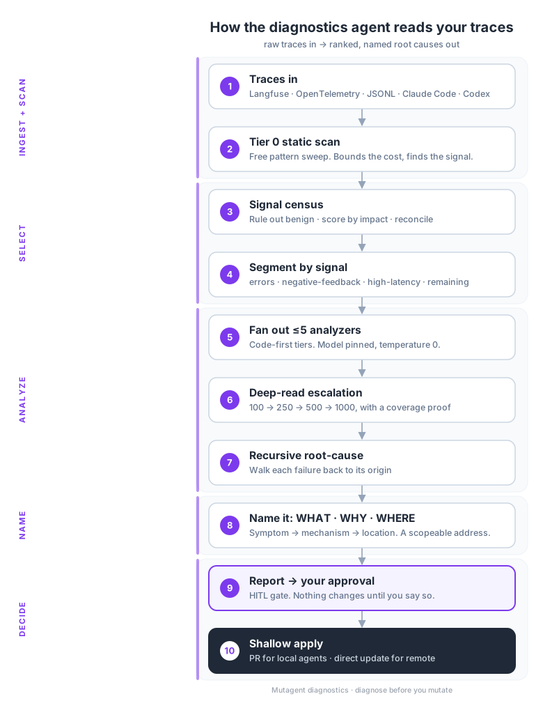The whole pipeline: scan to bound cost, census and segment to find what matters, fan out analyzers, walk each failure to its origin, name it on three axes, and hand you the decision.

Step one: bound the cost before you spend it

The first thing that runs is not a model. It is a static scan.

A language model reading every trace in your history is the most expensive way to start, and most of that spend is wasted on traces that are fine. So before any LLM call, a Tier 0 pass does a pattern-match sweep across the raw traces: count the error markers, the latency outliers, the cost spikes, the low-score and negative-feedback signals. Milliseconds, no tokens.

That scan does two jobs. It bounds the token budget for everything downstream, and it surfaces where the signal actually is. You do not deep-read a clean trace. You deep-read the places where something is wrong.

The tradeoff is explicit: a static scan can only catch what it can pattern-match. It will miss a semantic failure that looks structurally clean. That is why the scan is a cost gate, not a verdict. It decides where to spend the expensive reading, never what the answer is. Anything Tier 0 cannot see gets caught later, by an analyzer that actually reads the trace.

Step two: the signal census, or how it decides what’s worth diagnosing

Here is where most tools cheat. They see a lot of one pattern, declare that the problem, and move on. The trap is that the loudest pattern is usually a benign artifact: a low tagging rate, a retry that resolved itself, a metric that looks scary and means nothing.

So before any hypothesis gets generated, the agent runs a full signal census. It enumerates every signal type present in the scoped traces, errors, negative feedback, low scores, latency spikes, API exhaustion, behavior deviations, and then it does three things in order.

First, a failure-validity gate rules out the benign ones. A low tagging rate is an observability artifact, not a failure, and it gets labeled “ruled out” in the census rather than chased. Second, the survivors get scored by impact times prevalence, not by raw frequency. A failure that happens rarely but breaks the output ranks above one that happens constantly and changes nothing. Third, after the deep read runs, the static ranking gets reconciled against what the analyzers actually found. The primary signal the report leads with is the one that survives all three filters, not the one that showed up most.

This is the step that earns the word diagnosis. A frequency count is not a diagnosis. A census that rules out the noise, scores the rest by impact, and confirms the winner against real evidence is.

Step three: segment the traces

You cannot run one analysis over three thousand mixed traces and get a clean answer. Retries, format violations, and timeouts are different failures with different origins, and folding them into one pass produces mush.

So the next step segments the traces into clusters. When the scan found real signal, it slices by that signal:

• an errors cluster, every trace carrying an error marker
• a negative-feedback cluster, traces with a thumbs-down or a normalized score at or below 0.4
• a high-latency cluster, traces over ten seconds that were not already errors
• a remaining cluster that catches whatever is left, so nothing silently drops out of scope

When there is no a-priori signal to cluster on, it falls back to a window-based split instead. Either way you end up with a handful of coherent groups, each holding traces that failed in a related way, and each one homogeneous enough that the analysis running over it is looking at one kind of failure at a time.

The clustering is deterministic. It is signal segmentation, not a learned embedding, and that matters: you can read the slice plan, see exactly why a trace landed where it did, and reproduce it. There is no black box deciding which bucket your failure belongs in.

Step four: fan out the analyzers

Each cluster gets its own analyzer, and the analyzers run in parallel. The fan-out is capped at five. Never more than five analyzers at once, no matter how many clusters the data could produce.

The cap is a deliberate ceiling on cost and complexity. Three thousand traces do not become three thousand reads, or even thirty. They become at most five focused analyses, each pointed at one coherent slice, each running on its own with a hard time budget of a few minutes. If a slice is empty, its analyzer is skipped and the decision is logged. You can see, after the fact, exactly how many analyzers ran and why.

Inside each analyzer the work is code-first, not model-first. It runs in tiers: a cheap pattern-match pass, then a match against a library of known failure shapes, then a structural analysis of the trajectory, and only then, for the deviations the cheap tiers could not explain, does it spend a language model. The model is the last resort, not the first reflex. Most of what an analyzer concludes, it concludes without an LLM call at all.

And the one place it does call a model, it pins the model and pins the temperature to zero. This sounds like a detail. It is not. An unpinned model at a default temperature was the single biggest source of run-to-run variance: the same traces produced different findings on Tuesday than on Wednesday, for no reason except sampling noise. Pinning the inference is what makes a diagnosis reproducible. Run it twice on the same traces and the findings line up instead of drifting. A diagnosis you cannot reproduce is an opinion with a progress bar.

Step five: how deep does it actually read?

The static scan sees every trace. The analyzers do not, and pretending otherwise would be the lie that sinks the whole thing.

Deep reading is the expensive part, so it escalates in rungs rather than trying to read everything at once. It starts at a hundred traces. If the evidence at a hundred is not yet sufficient to ground the findings, it climbs to two hundred and fifty, then five hundred, then a thousand, and a thousand is the ceiling. Each rung carries its own time budget, from ten minutes at the smallest up to thirty at the largest, and the run stops the moment any active budget trips. When it stops, it emits the findings it has and raises a banner saying so. It never silently truncates and pretends it read more than it did.

Notice what is not in that list: a cost cap is defined but turned off by default. The design choice there is that this tool is trace-hungry, not cost-shy. The thing that destroys a diagnosis is reading too little and overgeneralizing from a thin sample, so the default bias is to read more, bounded by trace count and wall-clock time, the two things the tool can measure reliably.

The honesty payoff comes at the end. Because the deep read is sampled, the report carries a coverage proof and a confidence grade: here is the population, here is how much I read, here is how confident that sample lets me be. Diagnosis that hides its own coverage is marketing. Diagnosis that shows it is something you can act on.

Step six: recursive root-cause analysis

This is the part that separates diagnosis from a dashboard.

A dashboard tells you what happened: error rate up, latency p95 blown, score down. The analyzer does not stop there. It walks the failure backward. The output is wrong, so why is the output wrong? Because the tool returned the wrong field. Why did the tool return the wrong field? Because the tool definition is ambiguous about which field to read. Why is the definition ambiguous? Each answer is a new question, and the chain keeps going until it reaches an origin, something that nothing upstream explains.

There is no fixed depth. A shallow failure bottoms out in two steps; a deep one takes five. The chain stops when it hits an origin, not when it hits a preset number of hops. And every link has to cite evidence: a specific message index in the trace, or a specific line in the code. A why-chain that cannot point at the trace is a guess, and the analyzer is not allowed to ship guesses as facts.

The tradeoff here is honesty over tidiness. Sometimes the chain reaches a point where the next step would need code the agent cannot see, or evidence the traces do not contain. When that happens the finding is flagged as a hypothesis pending source, not dressed up as a confirmed root cause. A confident wrong diagnosis costs more than an honest “this is where the trail goes cold.”

03Mutagent Use CaseDiagnostics A failure-mode scan that finds root causes, not a wall of logs. Every finding is traced to a step and an origin, and ranked by impact. IN production traces    OUT ranked root causes · failure index Explore

The three axes: what, why, where

Every finding lands classified on three axes. This is the spine of the whole system, so it is worth being precise about what each one carries.

• WHAT is the symptom: wrong output, missing output, a loop, a latency spike, a cost overshoot, a format violation, a hallucination, a user complaint, a low score, missing context.
• WHY is the mechanism: an underspecified prompt, an overspecified one, a tool misused, a tool missing, a context window overflow, a provider limit, stale data, a lost handoff, a dependency failure.
• WHERE is the location: the system prompt, a tool definition, the agent config, the routing config, upstream data, the provider side, the harness, the user input.

“Wrong output” alone is useless. You cannot act on it. “Wrong output, because the tool was misused, located in the tool definition” is a fix you can scope. The three axes turn a symptom into an address.

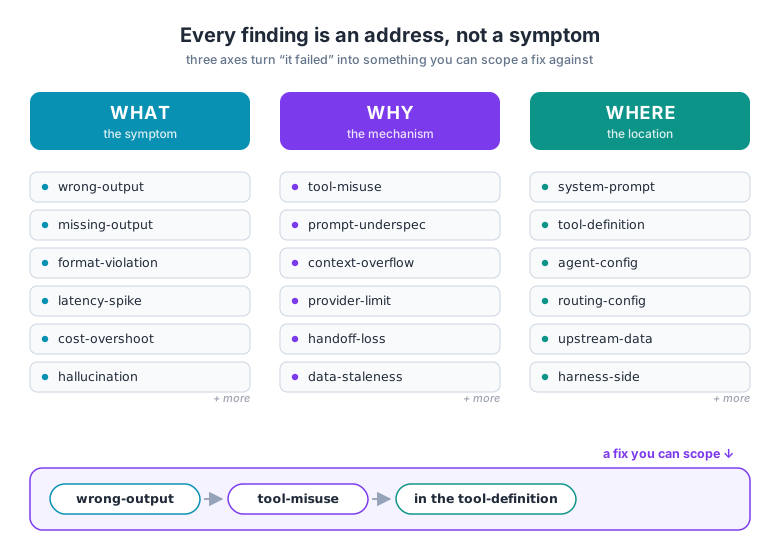A symptom you cannot place is a symptom you cannot fix. WHAT, WHY, and WHERE turn “wrong output” into an address.

The axes are constant. The category values are not. Diagnosing an agent, the WHAT values are the agent-failure modes above. Diagnosing a prompt, the WHAT values swap to the prompt taxonomy: instruction ambiguity, reasoning gaps, and the rest. The frame stays; the vocabulary adapts to what you are diagnosing. That is deliberate. The discipline is the three-axis structure, not any single list of labels.

This is also why you can only fix what you can name. A failure with no name is a vibe, and you cannot write a regression test against a vibe. Once a failure has a WHAT, a WHY, and a WHERE, it becomes a thing you can test for, a thing the next run recognizes, a thing the eval system can grow around. Every named failure class the agent confirms gets remembered and matched first on the next run, so the taxonomy compounds instead of starting cold each time.

The report, and the part where you stay in charge

The findings render into a report: an entity card for the agent under diagnosis, the signal census with its rule-outs visible, and one tab per finding carrying its taxonomy, its evidence, its why-chain, its assumptions, and a ranked set of remedies. The remedies are ranked by cost against correctness, the cheap high-confidence fix first.

Then it stops and waits for you. Nothing changes without your approval. You read the report, you pick the remedies you want, and you copy your decisions back as the approval. Only then does anything get applied.

Applying the fix: a PR or a direct update

When you approve, an apply agent spawns to land the change. What that looks like depends on where the target agent lives.

For a local agent, the kind defined by files in your repo, the apply runs on an isolated git worktree and opens a pull request. Your working checkout is never touched. You review the PR like any other and you merge it or you do not. For a remote agent on a target platform, the apply updates the agent directly on that platform through an idempotent write, so retrying it is safe.

This is a shallow apply, and the word matters. The agent diagnoses, names, and proposes. It can land the change once you approve it. It does not decide on its own that a change is worth making. The boundary is firm: the machine does the reading and the writing, the engineer owns the judgment. That is not a limitation we are apologizing for. It is the line we hold on purpose.

Why this is diagnosis and not the alternatives

Four things in this pipeline are doing the work that search, dashboards, and chat cannot.

1. It censuses before it concludes. Ruling out the benign-but-loud signal and scoring the rest by impact is what keeps the diagnosis off the obvious-but-wrong answer.
2. It reads across the dataset, with its coverage on the table. Segmentation is what lets a finding say “this origin appears across the cluster” instead of “this one run broke,” and the coverage proof is what lets you trust the sample it read.
3. It walks to an origin, not a symptom. The recursive why-chain is the difference between “latency is up” and “latency is up because the context window keeps overflowing because of a specific upstream choice.” You cannot fix the first. You can fix the last.
4. It names every failure on three axes. A symptom you cannot name is a symptom you cannot test, cannot remember, and cannot hand to a fix. The taxonomy is what makes the rest mechanical.

Optimization across all your production traces is a research problem, not a query you run and not a prompt you hand a coding assistant. Diagnose first. Name the origin. Then, and only then, change something, with your hand on the approval.

You can run it today. Point it at Langfuse, OpenTelemetry, raw JSONL, or your Claude Code and Codex session logs, and ask it to diagnose your agents.